


|
|
|
|
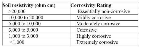
Soil resistivity is a function of soil moisture and the concentrations of ionic soluble salts and is considered to be most comprehensive indicator of a soil’s corrosivity. Typically, the lower the resistivity, the higher will be the corrosivity as indicated in the following Table. (reference)
Corrosivity ratings based on soil resistivity
Since ionic current flow is associated with soil corrosion reactions, high soil resistivity will arguable slow down corrosion reactions. Soil resistivity generally decreases with increasing water content and the concentration of ionic species.
Field soil resistivity measurements are most often conducted using the Wenner four-pin method and a soil resistance meter. The Wenner method requires the use of four metal probes or electrodes, driven into the ground along a straight line, equidistant from each other, as shown in the following Figure. Soil resistivity is a simple function derived from the voltage drop between the center pair of pins, with current flowing between the two outside pins.
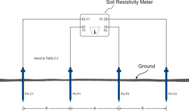
Wenner four pin soil resistivity test set-up
An alternating current from the soil resistance meter causes current to flow through the soil, between pins C1 and C2. The voltage or potential is then measured between pins P1 and P2. The meter then registers a resistance reading. Resistivity of the soil is then computed from the instrument reading, according to the following formula:
![]()
where:
ρ is the soil resistivity (ohm-centimeters)
A is the distance between probes (centimeters)
R is the soil resistance (ohms), instrument reading
π equals 3.1416
The resistivity values obtained represent the average resistivity of the soil to a depth equal to the pin spacing. Resistance measurements are typically performed to a depth equal to that of the buried system (pipeline) being evaluated. Typical probe spacing is in increments of 0.8 m (2.5 ft).
If the line of soil pins used when making four-pin resistivity measurements is closely parallel to a bare underground pipeline or other metallic structure, the presence of the bare metal may cause the indicated soil resistivity values to be lower than it actually is. Because a portion of the test current will flow along the metallic structure rather than through the soil, measurements along a line closely parallel to pipelines should be avoided.
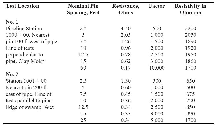
When making soil resistivity measurements along a pipeline, for example, it is good practice to place the line of the pins perpendicular to the pipeline with the nearest pin at least 4.5 meters from the pipe or even further, if space permits. Soil resistivity data taken by the four-pin method should be recorded in tabular form for convenience in calculating resistivity and evaluating results obtained. The tabular arrangement may be as shown here.
Format for recording soil resistivity measurements
With experience, much can be learned about the soil structure by inspecting series of readings to increasing depths. The recorded values from four-pin resistivity measurements can be misleading unless it is remembered that the soil resistivity encountered with each additional depth increment is averaged, in the test, with that of all the soil in the layers above. The indicated resistivity to a depth equal to any given pipe spacing is a weighted average of the soils from the surface to that depth. Trends can be illustrated best by inspecting the sets of soil resistivity readings such as in the following example.
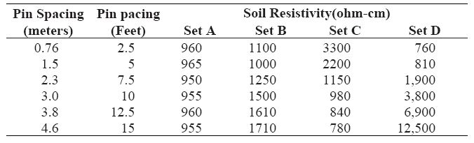
The first set of data, Set A, represents a uniform soil conditions. The average of the readings shown (~960 ohm-cm) represents the effective resistivity that may be used for design purposes for impressed current groundbeds or galvanic anodes.
Data Set B represents low-resistivity soils in the first few feet. There may be a layer of somewhat less than 1000 ohm-cm around the 1.5 meters depth level. Below 1.5 meters, however, higher-resistivity soils are encountered. Because of the averaging effect mentioned earlier, the actual resistivity at 2.3 meters deep would be higher than the indicated 1250 ohm-cm and might be in the order of 2500 ohm-cm or more.
Even if anodes were placed in the lower-resistivity soils, there would be resistance to the flow of current downward into the mass of the earth. If designs are based on the resistivity of the soil in which the anodes are placed, the resistance of the completed installation will be higher than expected. The anodes will perform best if placed in the lower resistance soil. The effective resistivity used for design purposes should reflect the higher resistivity of the underlying areas. In this instance, where increase is gradual, using horizontal anodes in the low-resistivity area and a figure of effective resistivity of ~2500 ohm-cm should result in a conservative design.
Data Set C represents an excellent location for anode location even though the surface soils have relatively high resistivity. It would appear from this set of data that anodes located >1.5 meters deep, would be in low-resistivity soil of ~800 ohm-cm, such a figure being conservative for design purposes. A lowering resistivity trend with depth, as illustrated by this set of data, can be relied upon to give excellent groundbed performance.
Data Set D is the least favorable of these sample sets of data. Low-resistivity soil is present at the surface but the upward trend of resistivity with depth is immediate and rapid. At the 2.3 meters depth, for example, the resistivity could be tens of thousands of ohm-centimeters. One such situation could occur where a shallow swampy area overlies solid rock. Current discharged from anodes installed at such a location will be forced to flow for relatively long distances close to the surface before electrically remote earth is reached.
As a result, potential gradients forming the area of influence around an impressed current groundbed can extend much farther than those surrounding a similarly sized groundbed operating at the same voltage in more favorable locations such as those represented by data Sets A and C.
In some areas, experience will show that soil resistivity may change markedly within short distances. A sufficient number of four-pin tests should be made in a groundbed construction area, for example, to be sure that the best soil conditions have been located. For groundbeds of considerable length (as may be the case with impressed current beds), four-pin tests should be taken at intervals along the route of the proposed line of groundbed anodes. If driven rod tests or borings are made to assist in arriving at an effective soil resistivity for design purposes, such tests should be made in enough locations to ascertain the variation in effective soil resistivity along the proposed line of anodes.
| (previous) | Page 7 of 10 | (next) |